최근에 ML/AI 쪽에 관심이 생기면서 책을 사서 공부까지 해보고 있는데, 옛날에는 import 해서 다른 학습 모델들을 가져다 썻었던 것에 비해서 책의 내용은 직접 구현하고 있으니 괴리감이 있었다.
기억이 희석되고 대체되기 보다는 기존의 내가 알던 것과 새로운 것을 비교해가면서 공부하려고 한다.
---------------------------------------------------------------------------------------------------------------------------------------------------------
|
1
2
3
4
5
6
7
8
9
10
11
12
13
14
15
16
17
18
19
20
21
22
23
|
from sklearn.datasets import load_iris
iris=load_iris()
iris.keys() #dict의 key values만 출력한다.
"""dict_keys(['data', 'target', 'frame', 'target_names', 'DESCR', 'feature_names', 'filename', 'data_module'])"""
iris.feature_names #특성 이름
""" ['sepal length (cm)', 'sepal width (cm)', 'petal length (cm)', 'petal width (cm)'] """
iris.target_names # 목표인, 종의 이름 (종 분류 .. 해야하니까)
""" array(['setosa', 'versicolor', 'virginica'], dtype='<U10') """
iris_pd = pd.DataFrame(iris.data, columns=iris.feature_names) # 분석을 위해 iris.data를 활용한 Dataframe을 만든다.
from sklearn.preprocessing import LabelEncoder
le = LabelEncoder() #labelencoder는 문자를 수치로 매핑한다.
le.fit(iris.target_names)
le.transform(['setosa', 'virginica']) #출력결과는? array([0, 2])
le.inverse_transform([1,2,0]) #수치를 문자로 매핑. 출력결과는 ? array(['versicolor', 'virginica', 'setosa'], dtype='<U10'))
iris_pd['species'] = le.inverse_transform(iris.target)
"""species라는 열을 추가한다. target은 숫자로 되어 있었으므로 inverse_transform을 통해 문자로 바꿀 수 있다."""
|
cs |
여기까지 하면, iris 데이터를 불러오고, keys()를 통해 어떤 데이터가 있는지,
feature로 무엇이 있고, target은 무엇으로 삼아야 하는지에 대해서 알 수 있따.
그리고 나서 feature를 column으로 한 Dataframe을 만들었다.
지금 와서 생각해보니 labelencoder 는 사용할 필요 없이 target 혹은 target_names를 통해 진행했어도 괜찮았을 것 같다.
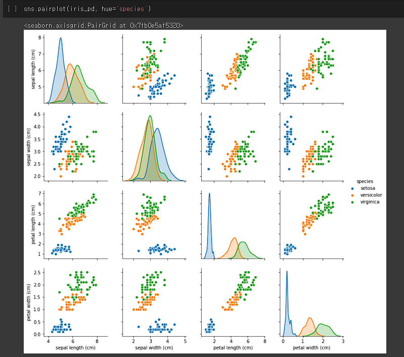
이런 식으로 pairplot을 통해 어떤 feature를 기준으로 종을 나눌지에 대해서 정한다.
Petal legnth랑 Petal width로 했다. 그래서...
|
1
2
3
4
5
6
7
8
9
10
11
12
|
feature_data = iris.data[:,2:] #Petal length, width 슬라이싱
from sklearn.tree import DecisionTreeClassifier #DecisionTreeClassifier를 가져온다. 쉽고 직관적이다.
iris_tree = DecisionTreeClassifier(max_depth = 2)
iris_tree.fit(feature_data, le.inverse_transform(iris.target)) #fit(feature, target) 보통 X_train, y_train 이라고 하는 그 것이다.
from graphviz import Source
from sklearn.tree import export_graphviz
Source(export_graphviz(iris_tree, feature_names=['length', 'width'],
class_names=iris.target_names,
rounded = True, filled=True))
|
cs |
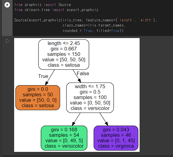
결정나무? 를 쉽게 이미지화 한 것. 기준이 length <= 2.45 등으로 나타나있다. featrue names에 length와 width 밖에 없는 이유는 fit에 들어가는 data가 위에서 슬라이싱한 데이터가 들어가기 때문..
더 제대로, trainset과 testset을 나누고 분류 모델을 만들어보자. 여기에, 모델의 성능을 파악해보자.
|
1
2
3
4
5
6
7
8
9
10
|
from sklearn.model_selection import train_test_split
feature_data = iris.data[:,2:]
X_train, X_test, y_train, y_test = train_test_split(feature_data, iris.target,
test_size = 0.2, random_state=13,
stratify = iris.target)
iris_tree = DecisionTreeClassifier(max_depth = 2, random_state = 13)
iris_tree.fit(X_train, y_train)
|
cs |
train_test_split을 통해서 주어진 데이터 중 일부를 test set으로 활용할 수 있다.
모델의 성능을 판단하는 함수로써
이렇게 accuracy_scory를 가져와서 얼마나 맞췄는지를 알 수 있다.
다른 성능 지표로
이렇게 하면 대표적인 분류 모델 성능 지표인 Confusitoin Matrix를 출력할 수 있다. 자세한 설명은
여기를 참조하면 더 좋은 설명이 될 것이다.
|
1
2
3
4
5
6
7
8
9
10
11
12
13
14
15
16
17
18
19
20
21
22
23
24
25
26
27
28
|
from matplotlib.colors import ListedColormap
import matplotlib.pyplot as plt
def plot_decision_regions(X, y, classifier, resolution=0.02):
markers = ('s', 'x', 'o', '^', 'v')
colors = ('red', 'blue', 'lightgreen', 'gray', 'cyan')
cmap = ListedColormap(colors[:len(np.unique(y))])
x1_min, x1_max = X[:, 0].min() - 1, X[:, 0].max() + 1
x2_min, x2_max = X[:, 1].min() - 1, X[:, 1].max() + 1
xx1, xx2 = np.meshgrid(np.arange(x1_min, x1_max, resolution), np.arange(x2_min, x2_max, resolution))
Z = classifier.predict(np.array([xx1.ravel(), xx2.ravel()]).T)
Z = Z.reshape(xx1.shape)
plt.contourf(xx1, xx2, Z, alpha=0.3, cmap=cmap)
plt.xlim(xx1.min(), xx1.max())
plt.ylim(xx2.min(), xx2.max())
for idx, cl in enumerate(np.unique(y)):
plt.scatter(x=X[y == cl, 0], y=X[y == cl, 1], alpha=0.8, c=colors[idx], marker=markers[idx], label=cl, edgecolor='black')
plt.figure(figsize=(10,6))
plot_decision_regions(X=X_train, y=y_train, classifier=iris_tree)
plt.xlabel('petal length [cm]')
plt.ylabel('petal width [cm]')
plt.legend(loc='upper left')
plt.show()
|
cs |
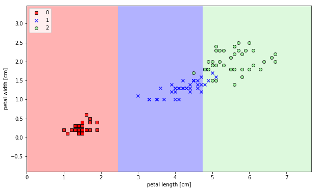
이렇게 출력이 된다. 위에서 보면 DecisionTreeClassifier(max_depth=2, random_state=13) 이라는 함수를 볼 수 있다.
max_depth는 말 그대로 Decision Tree의 깊이를 나타내는 것이다.
(random_state는 학습하는 데에 있어서 비교하기 편하게 일정한 값을 출력할 수 있도록 하는 것이라고 이해했다.)
만약에 Decision Tree의 깊이를 4로 한다면?
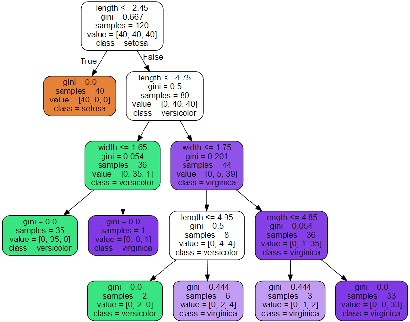
많이 복잡해졌다.... 해당 모델의 점수는?
하지만 위와 같은 overfitting 문제가 발생한다.
decisiontree의 깊이를 너무 깊게 하면 모델의 성능 자체는 올라갈 수 있어도, overfitting 문제가 발생할 수 잇음에 주의해야한다.
'Coding' 카테고리의 다른 글
| 과거 정리 - Untitled4.ipynb(타이타닉, 결정나무, pd.cut(), 결측치 처리 등) (0) | 2022.07.03 |
|---|---|
| 과거 정리 - Untitled2.ipynb(Boston, .corr(), rmse, scatter, .drop) (0) | 2022.06.28 |
| 과거 정리 - Untitled0.ipynb (import, plt 등) (0) | 2022.06.27 |
| ubuntu 제거 후 grub 커맨드 창 해결 방법 (UEFI) (+CMD 먹통 해결) (0) | 2022.06.25 |
| [python] KBO 기록실 크롤링 - 3 (0) | 2022.05.30 |


